Confused by data warehouse tool lists? This guide breaks down warehouse platforms, ETL/ELT, CDC, transformation, and governance tools so you can choose the right stack without overbuying.

Compare the best Oracle to PostgreSQL migration tools in 2026 for low-downtime cutovers, including BladePipe, Ora2Pg, Oracle GoldenGate, AWS DMS, and Qlik Replicate.
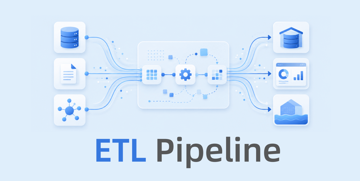
Learn what an ETL pipeline is, when to use it, and how to set one up with minimal coding, plus a comparison of today's common ETL tools.

Learn what data connectors are, how they work, the main connector types, common examples, and what to evaluate when choosing connectors for migration, replication, and real-time sync.
Learn why Oracle BLOB CDC is difficult, how LogMiner handles LOB changes, and the 5 technical challenges behind real-time Oracle BLOB replication.
Need to recommend tools for data replication in SQL databases? Compare 8 proven SQL database replication tools for real-time CDC, migration, and sync.
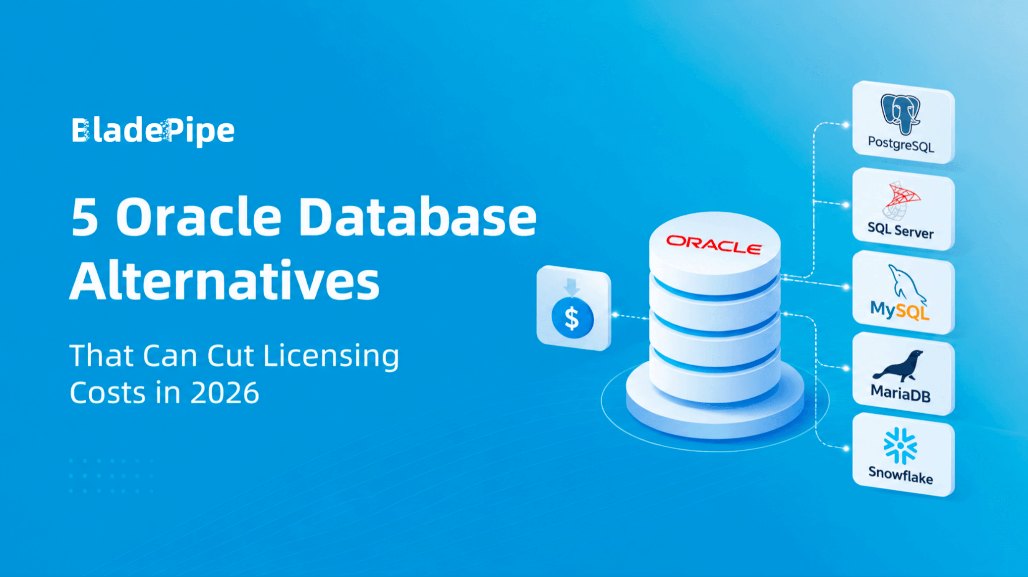
Compare 5 Oracle database alternatives including PostgreSQL, SQL Server, MySQL, MariaDB, and Snowflake, and learn how to migrate with lower costs.
A startup-focused comparison of Fivetran alternatives (Airbyte, Estuary, Stitch, Meltano, Hevo, Debezium, BladePipe) with verified pricing models, free tiers, and setup requirements.
Compare Debezium, Airbyte, Fivetran, Stitch, and BladePipe across pricing, latency, ops overhead, data consistency, and deployment to pick the right CDC/ELT tool for your stack.